Showing posts with label Finite Element (FE). Show all posts

Monday, October 10, 2011

deal.II Homepage

deal.II Homepage: A Finite Element Differential Equations Analysis Library - October 9th, 2011: deal.II 7.1 released

What is deal.II? 

deal.II is a C++ program library targeted at the computational solution of partial differential equations using adaptive finite elements. It uses state-of-the-art programming techniques to offer you a modern interface to the complex data structures and algorithms required. 
The main aim of deal.II is to enable rapid development of modern finite element codes, using among other aspects adaptive meshes and a wide array of tools classes often used in finite element program. Writing such programs is a non-trivial task, and successful programs tend to become very large and complex. We believe that this is best done using a program library that takes care of the details of grid handling and refinement, handling of degrees of freedom, input of meshes and output of results in graphics formats, and the like. Likewise, support for several space dimensions at once is included in a way such that programs can be written independent of the space dimension without unreasonable penalties on run-time and memory consumption. 
deal.II is widely used in many academic and commercial projects. For its creation, its principal authors have received the 2007 J. H. Wilkinson Prize for Numerical Software. It is also part of the industry standard SPEC CPU 2006 benchmark suite used to determine the speed of computers and compilers, and comes pre-installed on the machines offered by the commercial Sun Grid program. 

deal.II emerged from work at the Numerical Methods Group at Universität Heidelberg, Germany, which is at the forefront of adaptive finite element methods and error estimators. Today, it is maintained by two of its original authors at Texas A&M University, and dozens of contributors and several hundred users are scattered around the world (see our credits page for a detailed list of people contributing to deal.II).

What deal.II can offer you? 

If you are active in the field of adaptive finite element methods, deal.II might be the right library for your projects. Among other features, it offers: 

Support for one, two, and three space dimensions, using a unified interface that allows to write programs almost dimension independent. 

Handling of locally refined grids, including different adaptive refinement strategies based on local error indicators and error estimators. Both h, p, and hp refinement is fully supported for continuous and discontinuous elements. 

Support for a variety of finite elements: Lagrange elements of any order, continuous and discontinuous; Nedelec and Raviart-Thomas elements of any order; elements composed of other elements. 

Parallelization on single machine through the Threading Build Blocks and across nodes via MPI. deal.II has been shown to scale to at least 16k processors. 

Extensive documentation: all documentation is available online in a logical tree structure to allow fast access to the information you need. If printed it comprises more than 500 pages of tutorials, several reports, and presently some 5,000 pages of programming interface documentation with explanations of all classes, functions, and variables. All documentation comes with the library and is available online locally on your computer after installation. 

Modern software techniques that make access to the complex data structures and algorithms as transparent as possible. The use of object oriented programming allows for program structures similar to the structures in mathematical analysis. 

A complete stand-alone linear algebra library including sparse matrices, vectors, Krylov subspace solvers, support for blocked systems, and interface to other packages such as Trilinos, PETSc and METIS.

Support for several output formats, including many common formats for visualization of scientific data.

Portable support for a variety of computer platforms and compilers.
Free source code under an Open Source license, and the invitation to contribute to further development of the library.

Tuesday, October 4, 2011

Numerical Math - The Finite Element Method (FEM)


From Landau [1], the finite element method (FEM) is explained as solving a PDE where the whole region or domain is subsectioned into smaller areas known as elements. Next an initial solution is formulated for the PDE in each of the elements.  The next step comes in the form of modifying the parameters of the initial formalization known as a best fit.

Pepper and Heinrich [2] open their FEM book by explaining that the method is a numerical formulation that solves physics and engineering models described by differential equations  (DEs). Similar to finite difference methods (FDM), FEM models a geometric region which is then broken up into a number of smaller subregions which results in a network known as a mesh. One difference between FDM and FEM includes mesh type (geometrically). The FDM requires that the network be made of orthogonal rows and columns (squares and rectangles) while the FEM does not require this limitation and can be, in fact, any shape such as triangles and/or quadrilaterals in two dimensions and tetrahedrons and/or hexahedrons in three dimensions.  Next, each FE is initialized with an approximate functions of the unknown variables for which to be solved. Expansions determine the variables approximations and appear as a linear or higher-order polynomials functions. These expansions, in turn, depend upon the geometric shape of the elements and location known as nodes. A second difference between FDM and FEM noted by Pepper and Heinrich [3] entails the solution method. The FEM integrates over each subregion then adds or connects them to make up the whole. This integration and summation engenders a set of finite linear equations per section which can then be solved utilizing linear algebra methods. Jiang [6] also discusses that FEM does not...

The network of elements and nodes or where these elements connect make up discrete systems such as a trusses, circuits, and fluid transport pipes [5]. In order to solve for the system variables such as displacements, electric potentials, and pressures, one can begin with a known and simple parameter such as

Hooke’s Law:

\begin{equation} F = \dfrac{\Delta L}{R} = E A \dfrac{\Delta L}{L} \end{equation}

Ohm’s Law:

\begin{equation} i = \dfrac{\Delta V}{R} = \dfrac{A}{\rho} \dfrac{\Delta V}{L} \end{equation}

Poiseuille’s Law:

\begin{equation} \dot{m} = \dfrac{\Delta p}{R} = \dfrac{\rho \pi D^4}{128 \mu} \dfrac{\Delta p}{L} \end{equation}

Jiang [6] notes that FEM has been utilized as one of the most general numerical techniques to solve DEs and done so with great success. Jiang even quotes Oden as

Perhaps no other family of approximation methods has had a greater impact on the theory and application of numerical methods during the twentieth century


In progress...to be continued.


References:

[1] O. C. Zienkiewicz, R. L. Taylor, and J. Z. Zhu. The Finite Element Method - It’s Basis and Fundamentals, 6th ed. Elsevier Butterworth-Heinemann, Burlington, MA. 2005

[1] R. H. Landau, M. J. Páez, and C. C. Bordeianu. A Survey of Computational Physics - Introductory Computational Science, Princeton University Press, Princeton, New Jersey. 2008

[2] D. W. Pepper and J. C. Heinrich. The Finite Element Method: Basic Concepts and Applications, Taylor & Francis Hemisphere Publishing Corporation,. 1992

[4] J. C. Heinrich and D. W. Pepper. The Intermediate Finite Element Method: Fluid Flow and Heat Transfer Applications, Taylor & Francis Hemisphere Publishing Corporation, Washington, DC. 1999

[5] G. Comini, S. D. Giudice and C. Nonino. Finite Element Analysis in Heat Transfer: Basic Formulation & Linear Problems, Taylor & Francis Hemisphere Publishing Corporation, Washington, DC. 1994

[6] B.-N. Jiang. The Least-Squares Finite Element Method: Theory and Applications in Computational Fluid Dynamics and Electromagnetics, Springer-Verlag, Berlin, Germany. 1998

[7] O. C. Zienkiewicz, R. L. Taylor, and P. Nithiarasu. The Finite Element Method for Fluid Dynamics, (Volume 3) 6th ed. Elsevier Butterworth-Heinemann, Burlington, MA. 2005


Friday, August 12, 2011

FD1D_HEAT_EXPLICIT - Time Dependent 1D Heat Equation, Finite Difference, Explicit Time Stepping

A reference on a finite difference solution of the time dependent 1D heat equation using explicit time stepping in MATLAB (also available are codes in C, C++, and Fortran 77 and 90. There are also other links to similar programs and methods. I try to repost many things as they do not last on the internet forever and this will prove to be an invaluable collection.

FD1D_HEAT_EXPLICIT - TIme Dependent 1D Heat Equation, Finite Difference, Explicit Time Stepping

FD1D_HEAT_EXPLICIT is a MATLAB program which solves the time-dependent 1D heat equation, using the finite difference method in space, and an explicit version of the method of lines to handle integration in time.

FD1D_HEAT_EXPLICIT is available in a C version, a C++ version, a FORTRAN77 version, a FORTRAN90 version and a MATLAB version.

Related Data and Programs:

FD1D_BURGERS_LAX, a MATLAB program which applies the finite difference method and the Lax-Wendroff method to solve the non-viscous time-dependent Burgers equation in one spatial dimension.

FD1D_BURGERS_LEAP, a MATLAB program which applies the finite difference method and the leapfrog approach to solve the non-viscous time-dependent Burgers equation in one spatial dimension.

FD1D_BVP is a MATLAB program which applies the finite difference method to a two point boundary value problem in one spatial dimension.

FD1D_HEAT_IMPLICIT is a MATLAB program which uses the finite difference method and implicit time stepping to solve the time dependent heat equation in 1D.

FD1D_HEAT_STEADY is a MATLAB program which uses the finite difference method to solve the steady (time independent) heat equation in 1D.

FD1D_PREDATOR_PREY is a MATLAB program which uses finite differences to solve a 1D predator prey problem.

FD1D_WAVE, a MATLAB program which applies the finite difference method to solve the time-dependent wave equation in one spatial dimension.

FEM_50_HEAT is MATLAB program which applies the finite element method to solve the 2D heat equation.

FEM1D is a MATLAB program which applies the finite element method, with piecewise linear basis functions, to a linear two point boundary value problem;

FEM1D_ADAPTIVE is a MATLAB program which applies the finite element method to a linear two point boundary value problem in a 1D region, using adaptive refinement to improve the solution.

FEM1D_NONLINEAR is a MATLAB program which applies the finite element method to a nonlinear two point boundary value problem in a 1D region.

FEM1D_PMETHOD is a MATLAB program which applies the p-method version of the finite element method to a linear two point boundary value problem in a 1D region.

FEM2D_HEAT is a MATLAB program which applies the finite element method to solve the 2D heat equation.

FREE_FEM_HEAT is a MATLAB program which applies the finite element method to solve the time dependent heat equation in an arbitrary triangulated 2D region.

HOT_PIPE is a MATLAB program which uses FEM_50_HEAT to solve a heat problem in a pipe.

HOT_POINT is a MATLAB program which uses FEM_50_HEAT to solve a heat problem with a point source.

Reference:

George Lindfield, John Penny,
Numerical Methods Using MATLAB,
Second Edition,
Prentice Hall, 1999,
ISBN: 0-13-012641-1,
LC: QA297.P45.

Source Code:

fd1d_heat_explicit.m, the MATLAB function which carries out the calculation;

function [ H, x, t ] = fd1d_heat_explicit ( xn, tn )

%*****************************************************************************80
%
%% FD1D_HEAT_EXPLICIT: Finite difference solution of 1D heat equation.
%
% Discussion:
%
% This program solves
%
% dUdT - k * d2UdX2 = F(X,T)
%
% over the interval [A,B] with boundary conditions
%
% U(A,T) = UA(T),
% U(B,T) = UB(T),
%
% over the time interval [T0,T1] with initial conditions
%
% U(X,T0) = U0(X)
%
% The code uses the finite difference method to approximate the
% second derivative in space, and an explicit forward Euler approximation
% to the first derivative in time.
%
% The finite difference form can be written as
%
% U(X,T+dt) - U(X,T) ( U(X-dx,T) - 2 U(X,T) + U(X+dx,T) )
% ------------------ = F(X,T) + k * ------------------------------------
% dt dx * dx
%
% or, assuming we have solved for all values of U at time T, we have
%
% U(X,T+dt) = U(X,T) + cfl * ( U(X-dx,T) - 2 U(X,T) + U(X+dx,T) ) + dt * F(X,T)
%
% Here "cfl" is the Courant-Friedrichs-Loewy coefficient:
%
% cfl = k * dt / dx / dx
%
% In order for accurate results to be computed by this explicit method,
% the cfl coefficient must be less than 0.5!
%
% Licensing:
%
% This code is distributed under the GNU LGPL license.
%
% Modified:
%
% 05 April 2010
%
% Author:
%
% John Burkardt
%
% Reference:
%
% George Lindfield, John Penny,
% Numerical Methods Using MATLAB,
% Second Edition,
% Prentice Hall, 1999,
% ISBN: 0-13-012641-1,
% LC: QA297.P45.
%
% Parameters:
%
% Input, integer XN, the number of points to use in the spatial dimension.
%
% Input, integer TN, the number of equally spaced points in the time dimension.
%
% Output, real H(XN,TN), the computed solution.
%
% Output, real X(XN), the spatial points.
%
% Output, real T(TN), the time points.
%
timestamp ( );
fprintf ( 1, '\n' );
fprintf ( 1, 'FD1D_HEAT_EXPLICIT:\n' );
fprintf ( 1, ' MATLAB version.\n' );
fprintf ( 1, '\n' );
fprintf ( 1, ' Compute an approximate solution to the time-dependent\n' );
fprintf ( 1, ' one dimensional heat equation:\n' );
fprintf ( 1, '\n' );
fprintf ( 1, ' dH/dt - K * d2H/dx2 = f(x,t)\n' );
%
% Heat coefficient.
%
k = 0.002;
%
% X values;
%
xmin = 0.0;
xmax = 1.0;
x = linspace ( xmin, xmax, xn );
dx = ( xmax - xmin ) / ( xn - 1 );
%
% T values;
%
tmin = 0.0;
tmax = 80.0;
dt = ( tmax - tmin ) / ( tn - 1 );
t = linspace ( tmin, tmax, tn );
%
% Check the CFL condition, have processor 0 print out its value,
% and quit if it is too large.
%
cfl = k * dt / dx / dx;

fprintf ( 1, '\n' );
fprintf ( 1, ' CFL stability criterion value = %f\n', cfl );

if ( 0.5 <= cfl ) fprintf ( 1, '\n' ); fprintf ( 1, 'FD1D_HEAT_EXPLICIT - Fatal error!\n' ); fprintf ( 1, ' CFL condition failed.\n' ); fprintf ( 1, ' 0.5 <= K * dT / dX / dX = %f\n', cfl ); error ( 'FD1D_HEAT_EXPLICIT' ); end % % Compute and save initial values. % h = initial_condition ( xn, x, t(1) ); h = boundary_conditions ( xn, x, t(1), h ); H = zeros ( tn, xn ); H(1,1:xn) = h(1:xn); % % Compute the values of H at the next time, based on current data. % L = 1 : xn - 2; C = 2 : xn - 1; R = 3 : xn; for i = 1 : tn - 1 h(C) = h(C) + cfl * ( h(L) - 2.0 * h(C) + h(R) ) + dt * rhs ( x(C), t(i) ); h = boundary_conditions ( xn, x, t(i+1), h ); H(i+1,1:xn) = h(1:xn); end % % Terminate. % fprintf ( 1, '\n' ); fprintf ( 1, 'FD1D_HEAT_EXPLICIT:\n' ); fprintf ( 1, ' Normal end of execution.\n' ); fprintf ( 1, '\n' ); timestamp ( ); return end function h = boundary_conditions ( xn, x, t, h ) %*****************************************************************************80 % %% BOUNDARY_CONDITIONS evaluates the boundary conditions. % % Licensing: % % This code is distributed under the GNU LGPL license. % % Modified: % % 02 April 2010 % % Author: % % John Burkardt % % Parameters: % % Input, integer XN, the number of nodes. % % Input, real X(XN), the node coordinates. % % Input, real T, the current time. % % Input, real H(XN), the current heat values. % % Output, real H(XN), the current heat values, after boundary % conditions have been imposed. % h(1) = 90.0; h(xn) = 70.0; return end function h = initial_condition ( xn, x, t ) %*****************************************************************************80 % %% INITIAL_CONDITION evaluates the initial condition. % % Licensing: % % This code is distributed under the GNU LGPL license. % % Modified: % % 05 April 2010 % % Author: % % John Burkardt % % Parameters: % % Input, integer XN, the number of nodes. % % Input, real X(XN), the node coordinates. % % Input, real T, the initial time. % % Output, real H(XN), the heat values at the initial time. % h(1:xn) = 50.0; return end function value = rhs ( x, t ) %*****************************************************************************80 % %% RHS evaluates the right hand side of the differential equation. % % Licensing: % % This code is distributed under the GNU LGPL license. % % Modified: % % 05 April 2010 % % Author: % % John Burkardt % % Parameters: % % Input, real X(*), the node coordinates. % % Input, real T, the current time. % % Output, real VALUE(*), the source term. % value = x; value = 0.0; return end function timestamp ( ) %*****************************************************************************80 % %% TIMESTAMP prints the current YMDHMS date as a timestamp. % % Licensing: % % This code is distributed under the GNU LGPL license. % % Modified: % % 14 February 2003 % % Author: % % John Burkardt % t = now; c = datevec ( t ); s = datestr ( c, 0 ); fprintf ( 1, '%s\n', s ); return end


run_and_plot.m, a MATLAB script that supplies input to the function and shows how to plot the results.

%% RUN_AND_PLOT runs the code and plots the results.
%
% Discussion:
%
% This script suggests how to call the code that solves the
% heat equation, and uses some data that is reasonable.
%
fprintf ( 1, '\n' );
fprintf ( 1, 'RUN_AND_PLOT:\n' );
fprintf ( 1, ' Run FD1D_HEAT_EXPLICIT.\n' );
fprintf ( 1, ' Plot the results.\n' );
%
% XN is the number of equally spaced nodes to use between 0 and 1.
%
xn = 21;
%
% TN is the number of equally spaced time points between 0 and 10.0.
%
tn = 201;
%
% Running the code produces an array H of temperatures H(t,x),
% and vectors x and t.
%
[ H, x, t ] = fd1d_heat_explicit ( xn, tn );
%
% Now make a plot of the data.
%
[ X, T ] = meshgrid ( x, t );

mesh ( X, T, H );
title ( 'H(X,T) by FD1D\_HEAT\_EXPLICIT' );
xlabel ( '-- X --' );
ylabel ( '-- Time --' );
zlabel ( '-- H(X,T) --' );

fprintf ( 1, '\n' );
fprintf ( 1, 'RUN_AND_PLOT:\n' );
fprintf ( 1, ' Normal end of execution.\n' );


plot.png, a PNG image of the solution, using the MESH command to emphasize the method of lines approach underlying the solution.


Wednesday, August 10, 2011

Gmsh: a three-dimensional finite element mesh generator with built-in pre- and post-processing facilities

This is some software I ran across in Ubuntu's SC. Haven't tried it, but give it a go!

Gmsh: a three-dimensional finite element mesh generator with built-in pre- and post-processing facilities

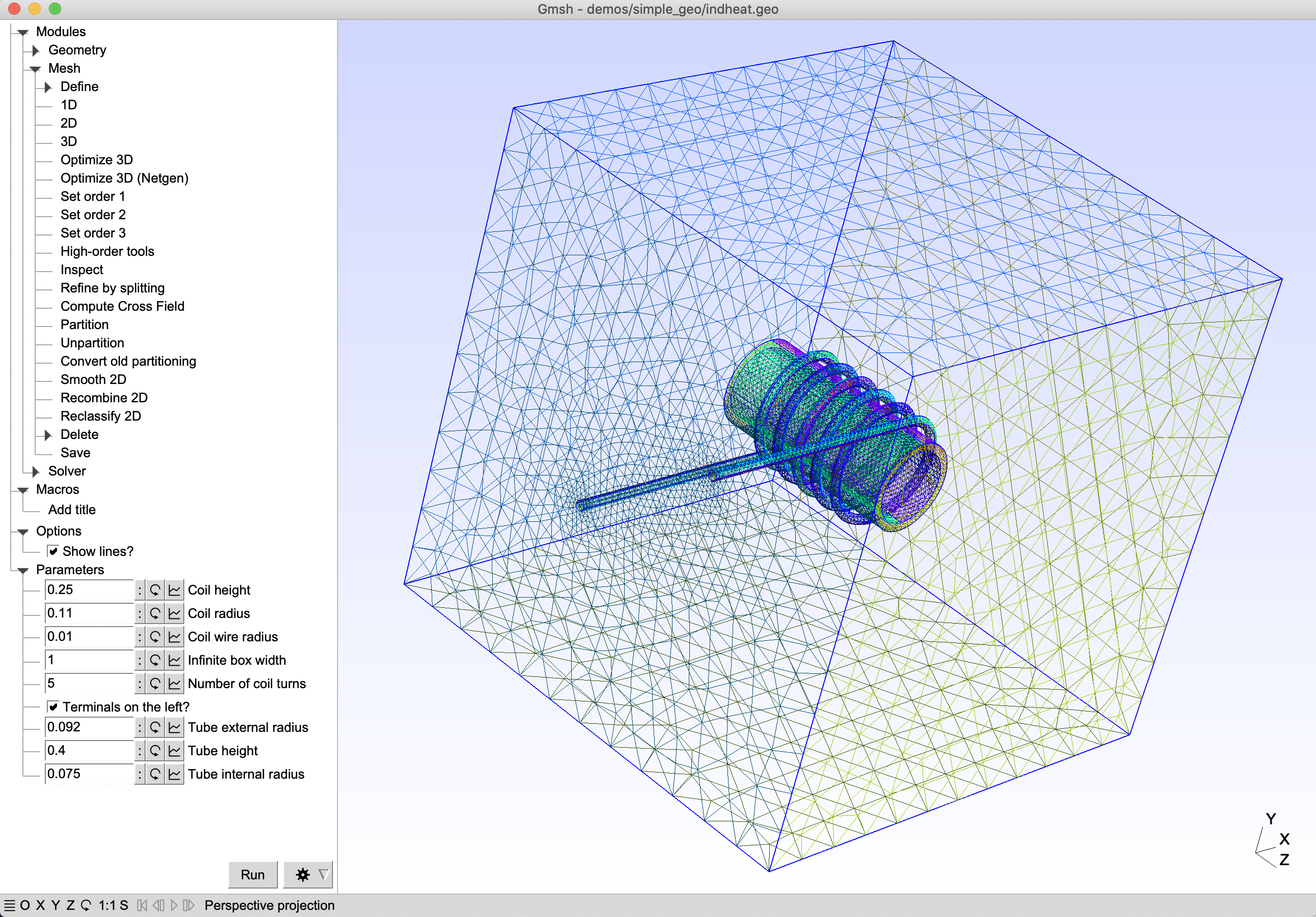
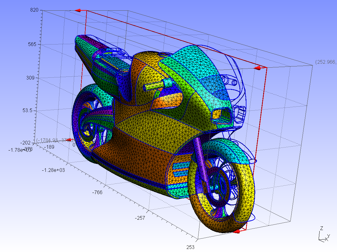
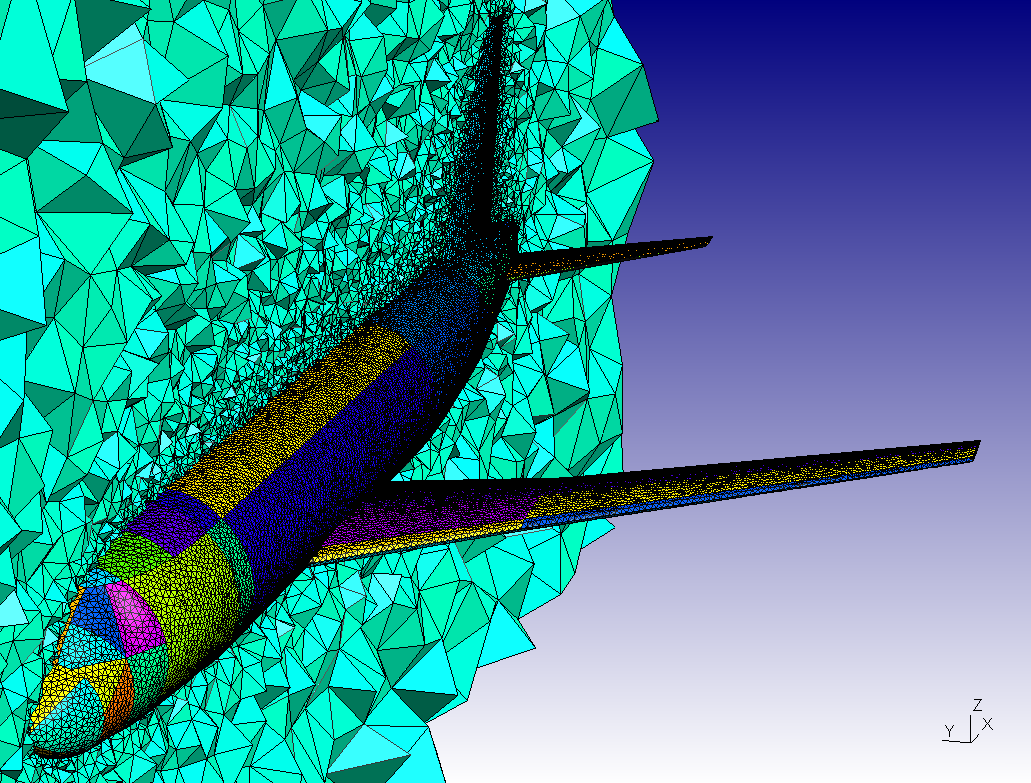
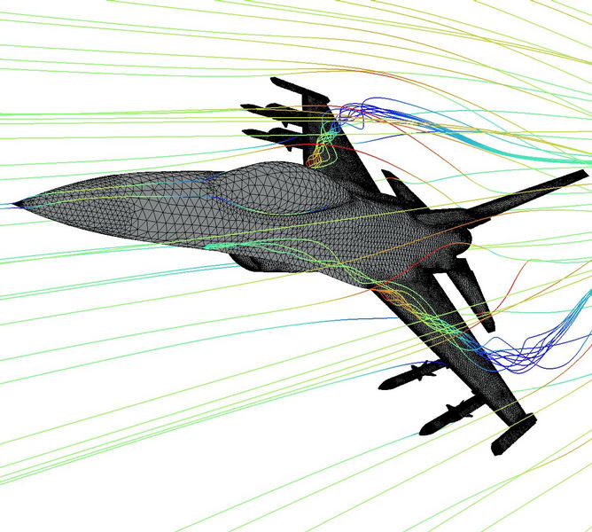
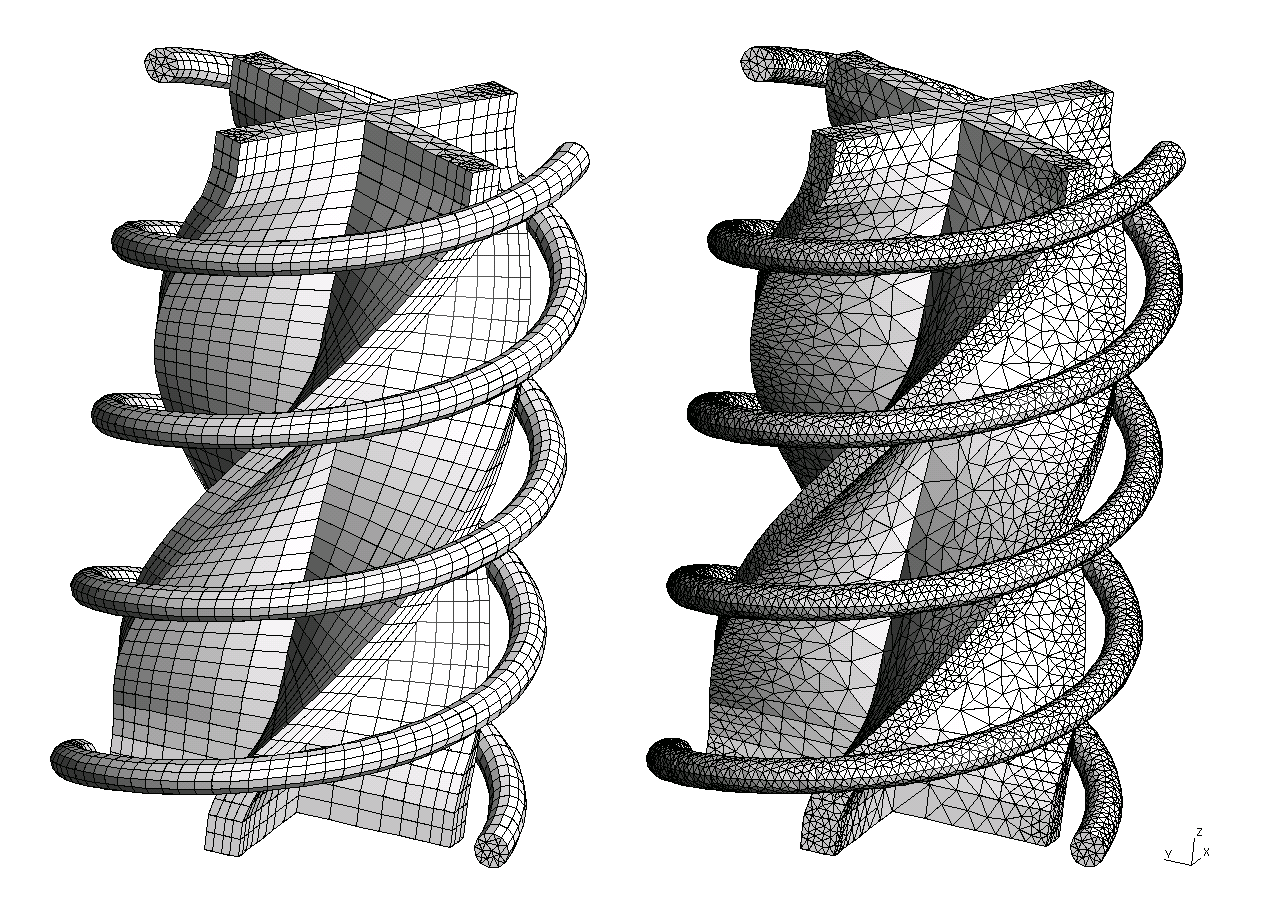
Gmsh is a 3D finite element grid generator with a build-in CAD engine and post-processor. Its design goal is to provide a fast, light and user-friendly meshing tool with parametric input and advanced visualization capabilities. Gmsh is built around four modules: geometry, mesh, solver and post-processing. The specification of any input to these modules is done either interactively using the graphical user interface or in ASCII text files using Gmsh's own scripting language.


Example screenshots from their website.